A Complete Guide to Parallel Axis Summation in Mojo

31 Aug, 2025

When working with multidimensional arrays on GPUs, one of the most common operations you'll encounter is axis summation. Axis summation is an algorithm that reducing a tensor along specific dimensions. Today, we'll explore two kind of implementations that demonstrate the power of shared memory parallel reduction, examining both axis=0 (column-wise) and axis=1 (row-wise) summation operations.

What is Axis Summation?

Before diving into the GPU implementation, let's establish what we mean by axis summation. Imagine you have a 2D matrix like this :

Matrix (8×16): Each element = row × 10 + column

svgviewer-output (2)-4

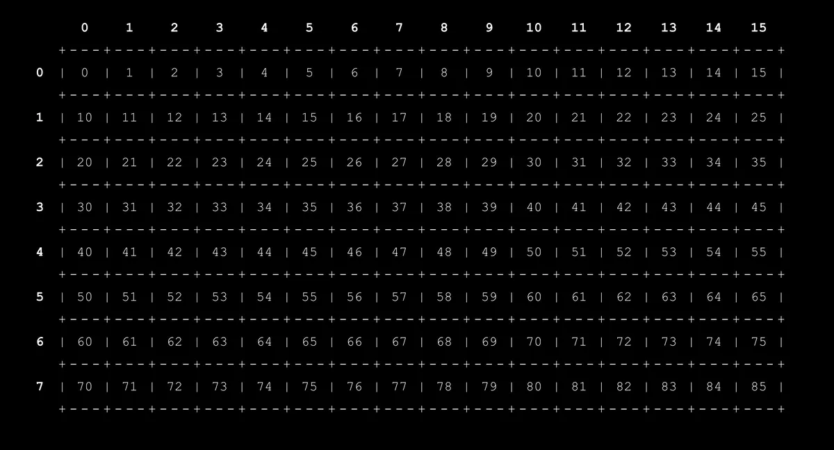
Axis Operations:

Axis=0 Sum (↓): Sum down each column → 16 results
[280, 288, 296, 304, ..., 368, 376, 384]
Axis=1 Sum (→): Sum across each row → 8 results
[120, 280, 440, 600, 760, 920, 1080, 1240]

Axis=0 Sum (Column-wise) : We sum down each column, collapsing the rows but keeping the columns. This gives us a result with 16 elements, one sum for each column.

Axis=1 Sum (Row-wise) : We sum across each row, collapsing the columns but keeping the rows. This gives us a result with 8 elements, one sum for each row.

The challenge in GPU programming is performing these reduction efficiently while leveraging parallel processing capabilities.

The Power of Shared Memory Reduction

Both implementations use a technique called shared memory parallel reduction. This approach is crucial for GPU efficiency because:

Shared memory is fast: It's much faster than global memory access
Parallel tree reduction: Multiple threads work together to reduce computation time from O(n) to O(log n)
Minimizes memory traffic: Data is loaded once, then processed entirely in fast shared memory

Let's examine how this works by walking through each implementation.

Impl. 1: Axis=0 Sum (Column-wise Reduction)

The first implementation tackles what's typically the more challenging case: summing along rows to produce column sums.

The Challenge: Strided Memory Access

# PHASE 1: Load data into shared memory
# Each thread loads one element from its assigned row in this column
# NOTE: This creates a stripped memory access pattern across threads
shared[tid] = input_tensor[tid, bid][0];

Here's why this is challenging: when threads within a block access input_tensor[tid, bid], they're accessing elements from different rows of the same column. In row-major layout, this means threads are accessing memory locations that are cols positions apart, a strided access pattern that's less optimal than consecutive access.

However, the beauty of shared memory reduction shines through: once we load the data into shared memory, the reduction algorithm becomes identical regardless of the loading pattern.

The Reduction Tree Algorithm

# PHASE 2: Parallel reduction - same algorithm as axis=1!
var stride = threads_per_block // 2;
while stride > 0:
    if tid < stride:
        # Each active thread adds its partner's value
        shared[tid] += shared[tid + stride];
    
    # Wait for all active threads to complete this round
    barrier();
    
    # Move to next level of the tree
    stride //= 2;

This is where the magic happens. The algorithm works like an upside-down binary tree:

Round 1: Thread 0 adds thread 4's value, thread 1 adds thread 5's value, etc.
Round 2: Thread 0 adds thread 2's value, thread 1 adds thread 3's value
Round 3: Thread 0 adds thread 1's value
Result: Thread 0 holds the final sum

The barrier() calls are crucial, they ensure all threads complete each round before proceeding to the next level.

Block and Thread Organization

ctx.enqueue_function[axis0_reduction_kernel](
    input_tensor,
    output_tensor,
    grid_dim=cols,                  # One block per column
    block_dim=threads_per_block,    # One thread per row
);

For axis=0 reduction, we launch 16 blocks (one per column), each with8 threads (one per row). Each block independently computes the sum of its assigned column.

Impl. 2: Axis=1 Sum (Row-wise Reduction)

The second implementation handles the more straightforward case: summing across columns to produce row sums.

The Advantage: Coalesced Memory Access

# PHASE 1: Load data into shared memory
# Each thread loads one element from its assigned column in this row
var loaded_value = input_tensor.load[1](bid, tid);
shared[tid] = loaded_value[0];

This access pattern is optimal for GPUs. When threads within a block access input_tensor[bid, tid], they're accessing consecutive memory locations within the same row. This coalesced access pattern maximizes memory bandwidth utilization.

Identical Reduction Logic

Once the data is loaded into shared memory, the reduction algorithm is identical to the axis=0 case:

# PHASE 2: Parallel reduction using the tree pattern
# This is exactly our standard shared memory reduction algorithm
var stride = threads_per_block // 2;
while stride > 0:
    if tid < stride:
        shared[tid] += shared[tid + stride];
    barrier();
    stride //= 2;

This demonstrates a key principle: the reduction algorithm is independent of the data loading pattern. Whether we load data in a strided or coalesced manner, once it's in shared memory, the tree reduction proceeds identically.

Block and Thread Organization

ctx.enqueue_function[axis1_reduction_kernel](
    input_tensor,
    output_tensor,
    grid_dim=rows,  # One block per row
    block_dim=threads_per_block,    # One thread per column
);

For axis=1 reduction, we launch 8 blocks (one per row), each with 16 threads (one per column). Each block independently computes the sum of its assigned row.

Key Design Principles and Best Practices

1. Shared Memory Allocation Strategy

var shared = stack_allocation[
    threads_per_block,
    Scalar[dtype],
    address_space=AddressSpace.SHARED,
]();

The shared memory is allocated statically with a size equal to the number of threads per block. This ensures each thread has its own slot in shared memory, preventing race conditions during the initial load phase.

2. Synchronization Points

The barrier() calls serve as synchronization points that ensure:

All threads complete data loading before reduction begins
All threads in each reduction round finish before moving to the next round
Memory consistency across threads within the block

3. Thread Divergence Management

if tid < stride:
    shared[tid] += shared[tid + stride];

As the reduction progresses, fewer threads remain active. This creates thread divergence within warps, but it's acceptable because the total number of inactive threads decreases exponentially, and the performance impact is minimal compared to the algorithmic benefits.

4. Memory Access Pattern Optimization

The axis=1 implementation benefits from coalesced memory access, while axis=0 must handle strided access. Both patterns are handled efficiently by loading data into shared memory first, then performing the reduction in the fast shared memory space.

Performance Considerations

Time Complexity: Both implementations achieve O(log n) time complexity for the reduction phase, compared to O(n) for sequential reduction. Memory Bandwidth: Axis=1 reduction typically performs better due to coalesced global memory access, while axis=0 reduction may have slightly lower bandwidth utilization due to strided access. Scalability: Both implementations scale well with problem size, as each block operates independently and the reduction tree depth grows logarithmically.

Complete Code Impl.

Now let's examine the complete implementation that put all these concepts into practice. I'll present both codes with additional explanatory comments that highlight the key technical decisions.

Impl. 1: Axis=0 Sum (Column-wise Reduction)

This implementation demonstrates how to handle the more challenging case of strided memory access while maintaining optimal reduction performance.

from gpu import thread_idx, block_idx, barrier
from gpu.host import DeviceContext
from layout import Layout, LayoutTensor
from math import iota
from gpu.memory import AddressSpace
from memory import stack_allocation
from testing import assert_equal

alias dtype = DType.float32;
alias rows = 8;
alias cols = 16;
alias threads_per_block = rows;
alias total_elements = rows * cols;

fn axis_sum() raises:
    """
    Complete demonstration of axis sum using only shared memory parallel reduction.
    We'll implement both axis=0 and axis=1 to show how the algorithm adapts.
    """
    print("AXIS SUM USING PURE SHARED MEMORY REDUCTION");
    print("="*50);
    print(String("Working with {}x{} tensor").format(rows, cols));
    print("Demonstrate axis=0 sum operations");

    var ctx = DeviceContext();

    # Create input tensor buffer
    var input_buffer = ctx.enqueue_create_buffer[dtype](total_elements);

    # Create output buffers for both axis operations
    var output_buffer = ctx.enqueue_create_buffer[dtype](cols);

    # Initialize with a clear pattern that makes verification easy
    with input_buffer.map_to_host() as host_data:
        for row in range(rows):
            for col in range(cols):
                idx = row * cols + col;
                # Create a pattern where each row has predictable sums
                host_data[idx] = Float32(row * 10 + col);
    
    # Zero the output buffers
    _ = output_buffer.enqueue_fill(0);

    # Create tensor views
    alias tensor_layout = Layout.row_major(rows, cols);
    alias InputTensor = LayoutTensor[dtype, tensor_layout, MutableAnyOrigin];
    var input_tensor = InputTensor(input_buffer);

    alias output_layout = Layout.row_major(cols);
    alias OutputTensor = LayoutTensor[dtype, output_layout, MutableAnyOrigin];
    var output_tensor = OutputTensor(output_buffer);

    var expected_buffer = ctx.enqueue_create_host_buffer[dtype](cols);
    ctx.synchronize();

    # Fill expected buffer with calculated values
    for i in range(cols):
        var expected: Float32 = 0.0;
        for j in range(rows):
            expected += Float32(j * 10 + i);
        expected_buffer[i] = expected;
    
    # Let's implement axis=0 sum (sum along rows, keep columns)
    column_wise_sum_shared_memory(
        ctx,
        input_tensor,
        output_tensor,
    );

    # Verify and display results
    with output_buffer.map_to_host() as output_buffer_host:
        print("\nout:", output_buffer_host);
        print("expected:", expected_buffer);

        for i in range(cols):
            assert_equal(output_buffer_host[i], expected_buffer[i]);
        
        print("✓ All assertions passed!");

fn column_wise_sum_shared_memory(
    ctx: DeviceContext,
    input_tensor: LayoutTensor[dtype, Layout.row_major(rows, cols), MutableAnyOrigin],
    output_tensor: LayoutTensor[dtype, Layout.row_major(cols), MutableAnyOrigin]
) raises:
    """
    Axis=0 Sum: Sum along rows (reduce rows, keep columns).

    This is more complex because we need to sum elements from different rows
    but the same column. The memory access pattern is less optimal, but
    shared memory reduction still works beautifully.    
    """
    print("\n" + "-"*30);
    print("IMPLEMENTING AXIS=0 SUM");
    print("-"*30);
    print("Strategy: Each block processes one column");
    print("Threads access elements from different rows, same column");
    print("Memory access is strided, but algorithm is still efficient");

    fn axis0_reduction_kernel(
        input_tensor : LayoutTensor[dtype, Layout.row_major(rows, cols), MutableAnyOrigin],
        output_tensor : LayoutTensor[dtype, Layout.row_major(cols), MutableAnyOrigin] 
    ):
        """
        Each thread block reduces one row.
        This is a direct application of our shared memory reduction pattern.
        """
        # Allocate shared memory for this blocks's reduction
        var shared = stack_allocation[
            threads_per_block,
            Scalar[dtype],
            address_space=AddressSpace.SHARED,
        ]();

        var tid = thread_idx.x;
        var bid = block_idx.x;

        # PHASE 1: Load data into shared memory
        # Each thread loads one element from its assigned row in this column
        # NOTE: This creates a strided memory access pattern across threads
        shared[tid] = input_tensor[tid, bid][0];

        # Synchronize before starting reduction
        barrier();

        # PHASE 2: Parallel reduction - same algorithm as axis=1!
        # The beauty of shared memory reduction: once data is in shared memory,
        # the reduction algorithm is identical regardless of how we loaded the data
        var stride = threads_per_block // 2;
        while stride > 0:
            if tid < stride:
                # Each active thread adds its partner's value
                shared[tid] += shared[tid + stride];
            
            # Wait for all active threads to complete this round
            barrier();

            # Move to next level of the tree
            stride //= 2;
        
        # PHASE 3: Write result
        # Thread 0 holds the final sum for this row
        if tid == 0:
            output_tensor[bid] = shared[0];
    
    print("Launching axis=0 kernel: 16 blocks x 8 threads");
    ctx.enqueue_function[axis0_reduction_kernel](
        input_tensor,
        output_tensor,
        grid_dim=cols,                  # One block per column
        block_dim=threads_per_block,    # One thread per row
    );

fn main() raises:
    axis_sum();

Impl. 2: Axis=1 Sum (Row-wise Reduction)

This implementation demonstrates the optimal case where memory access patterns align perfectly with GPU architecture.

from gpu import thread_idx, block_idx, barrier
from gpu.host import DeviceContext
from layout import Layout, LayoutTensor
from math import iota
from gpu.memory import AddressSpace
from memory import stack_allocation
from testing import assert_equal, assert_almost_equal

alias dtype = DType.float32;
alias rows = 8;
alias cols = 16;
alias total_elements = rows * cols;

fn axis_sum() raises:
    """
    Complete demonstration of axis sum using only shared memory parallel reduction.
    We'll implement both axis=0 and axis=1 to show how the algorithm adapts.
    """
    print("AXIS SUM USING PURE SHARED MEMORY REDUCTION");
    print("="*50);
    print(String("Working with {}x{} tensor").format(rows, cols));
    print("Will demonstrate axis=1 sum operations");

    var ctx = DeviceContext();

    # Create input tensor buffer
    var input_buffer = ctx.enqueue_create_buffer[dtype](total_elements);

    # Create output buffers for both axis operations
    var output_buffer = ctx.enqueue_create_buffer[dtype](rows);

    # Initialize with a clear pattern that makes verification easy
    with input_buffer.map_to_host() as host_data:
        for row in range(rows):
            for col in range(cols):
                idx = row * cols + col;
                # Create a pattern where each row has predictable sums
                host_data[idx] = Float32(row * 10 + col);

    # Zero the output buffers
    _ = output_buffer.enqueue_fill(0);

    # Create tensor views
    alias tensor_layout = Layout.row_major(rows, cols);
    alias InputTensor = LayoutTensor[dtype, tensor_layout, MutableAnyOrigin];
    var input_tensor = InputTensor(input_buffer);

    alias output_layout = Layout.row_major(rows);
    alias OutputTensor = LayoutTensor[dtype, output_layout, MutableAnyOrigin];
    var output_tensor = OutputTensor(output_buffer);

    var expected_buffer = ctx.enqueue_create_host_buffer[dtype](rows);
    ctx.synchronize();

    # Fill expected buffer with calculated values
    for i in range(rows):
        var expected: Float32 = 0.0;
        for j in range(cols):
            expected += Float32(i * 10 + j);
        expected_buffer[i] = expected;

    # Let's implement axis=1 sum (sum along columns, keep rows)
    row_wise_sum_shared_memory(
        ctx,
        input_tensor,
        output_tensor
    );

    # Verify and display results
    with output_buffer.map_to_host() as output_buffer_host:
        print("\nout:", output_buffer_host);
        print("expected:", expected_buffer);

        for i in range(rows):
            assert_equal(output_buffer_host[i], expected_buffer[i]);
        
        print("✓ All assertions passed!");

fn row_wise_sum_shared_memory(
    ctx: DeviceContext, 
    input_tensor : LayoutTensor[dtype, Layout.row_major(rows, cols), MutableAnyOrigin], 
    output_tensor : LayoutTensor[dtype, Layout.row_major(rows), MutableAnyOrigin]
) raises:
    """
    Axis=1 Sum: Sum along columns (reduce columns, keep rows)
    This is the "easy" case because each row can be processed independently.
    Memory access pattern: threads access consecutive memory locations.
    """

    print("\n" + "-"*30);
    print("IMPLEMENTING AXIS=1 SUM");
    print("-"*30);
    print("Strategy: Each block processes one row independently");

    alias threads_per_block = cols; # One thread per column in the row

    fn axis1_reduction_kernel(
        input_tensor: LayoutTensor[dtype, Layout.row_major(rows, cols), MutableAnyOrigin], 
        output_tensor: LayoutTensor[dtype, Layout.row_major(rows), MutableAnyOrigin]
    ):
        """
        Each thread block reduces one row.
        This is a direct application of our shared memory reduction pattern.
        """
        # Allocate shared memory for this block's reduction
        var shared = stack_allocation[
            threads_per_block,
            Scalar[dtype],
            address_space=AddressSpace.SHARED,
        ]();

        var tid = thread_idx.x;     # Which column this thread handles
        var bid = block_idx.x;      # Which row this block handles

        # PHASE 1: Load data into shared memory
        # Each thread loads one element from its assigned column in this row
        var loaded_value = input_tensor.load[1](bid, tid);
        shared[tid] = loaded_value[0];
        
        # Synchronize to ensure all data is loaded before reduction begins
        barrier();

        # PHASE 2: Parallel reduction using the tree pattern
        # This is exactly our standard shared memory reduction algorithm
        var stride = threads_per_block // 2;
        while stride > 0:
            if tid < stride:
                # Each active thread adds its partner's value
                shared[tid] += shared[tid + stride];
            
            # Wait for all active threads to complete this round
            barrier();

            # Move to next level of the tree
            stride //= 2;
        
        # PHASE 3: Write result
        # Thread 0 holds the final sum for this row
        if tid == 0:
            output_tensor[bid] = shared[0];
        
    print("Launching axis=1 kernel: 8 blocks x 16 threads");
    ctx.enqueue_function[axis1_reduction_kernel](
        input_tensor,
        output_tensor,
        grid_dim=rows,  # One block per row
        block_dim=threads_per_block,    # One thread per column
    );

fn main() raises:
    axis_sum();

Conclusion

These implementations showcase fundamental GPU programming concepts that extend far beyond axis summation. The shared memory parallel reduction pattern appears in numerous algorithms including:

Matrix reductions (finding max, min, mean)
Dot products and matrix multiplication building blocks
Histogram computation
Prefix sum operations

The key insight is that by loading data into shared memory and applying tree-based reduction, we can achieve efficient parallel computation regardless of the initial memory access pattern. The algorithm's elegance lies in its separation of concerns: data loading adapts to the specific axis requirements, while the reduction logic remains consistent and optimal.

Understanding these patterns will serve you well as you tackle more complex GPU computing challenges, from machine learning workloads to scientific computing application